Introduction to Diffusion Models

May 27, 2024 | min | Jean-Baptiste Bouvier

Diffusion models have reached state-of-the-art performance in terms of image and video generation. Thus, most of the models available online focus on these difficult tasks which require complex code inaccessible to the novice. Instead, in this post I will focus on the implementation of a simple diffusion model in Python in just 100 lines of code! This mininal implementation makes understanding diffusion models much easier! All the codes mentioned in this post are available on GitHub.

What are diffusion models?

Diffusion models belong to the class of generative machine learning as they can create new content. In short, diffusion models learn to iteratively remove noise from the data until obtaining a clean sample. The generation process starts from a purely stochastic signal, a white noise. Then, a trained diffusion model can iteratively decrease the noise level of this data until converging to a sample of a desired distribution (for instance images of bikes).

There are plenty of good resources explaining in great detail how diffusion models work, such as Lilian Weng's blog post or even Wikipedia. However, the understanding brought by these excellent resources is not enough to actually code a diffusion model. Here I will focus on extremely simple models allowing to understanding how to code your first diffusion model.

How to implement a diffusion model in 100 lines of Python?

The simplest diffusion code is simple_1Diffusion.py, which you can find in the codes folder of the GitHub repo. This code implements a basic diffusion model for 1D data and is self-contained in 100 lines of Python!

Libraries

import torch
import random
import numpy as np
import torch.nn as nn
import matplotlib.pyplot as plt

Data distribution

mu_data = 1.
sigma_data = 0.01 

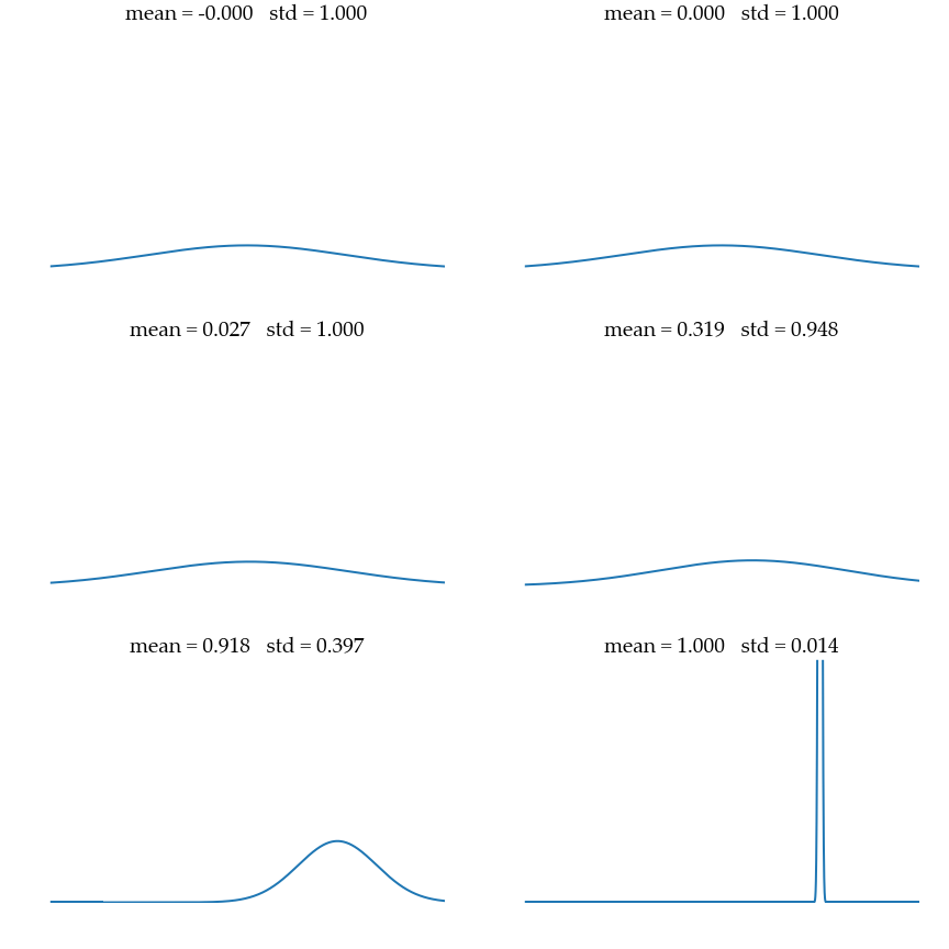
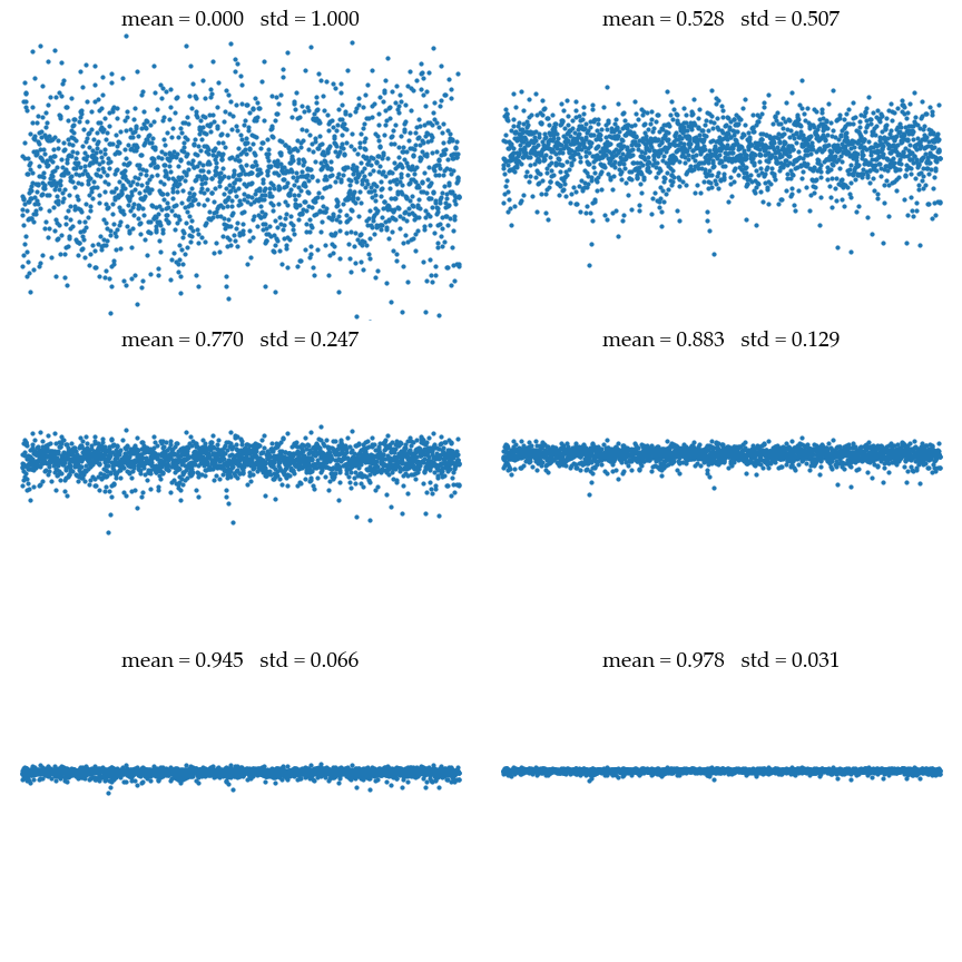
The goal will be to recover this data distribution from a unit Gaussian noise of mean $\mu_{noise} = 0$ and std $\sigma_{noise} = 1$ as illustrated below.

Hyperparameters

lr = 1e-3 
batch_size = 32 
nb_epochs = 1000
sigma_min = sigma_data/10 
sigma_max = 1. 
N = 10 # number of noise scales 
rho = 7 # log normal scale
Sigmas = (sigma_max**(1/rho) + torch.arange(N)*(sigma_min**(1/rho) - sigma_max**(1/rho))/(N-1))**rho
Sigmas = torch.cat((Sigmas, torch.tensor([0.])), dim=0)
test_size = 1000  

Denoiser

class Denoiser(nn.Module):
  def __init__(self, width):
    super().__init__()
    self.net = nn.Sequential(nn.Linear(1+1, width), nn.ReLU(),
			  nn.Linear(width, width), nn.ReLU(),
			  nn.Linear(width, 1) )
  
  def forward(self, x, sigma):
    s = sigma*torch.ones_like(x)
    return self.net( torch.cat((x, s), dim=1) )   

denoiser = Denoiser(32)  

Training

losses = np.zeros(nb_epochs)
optimizer = torch.optim.SGD(denoiser.parameters(), lr)

for epoch in range(nb_epochs):
  id_sigma = random.randint(0, N-1) 
  sigma = Sigmas[id_sigma]
  y = torch.randn((batch_size,1))*sigma_data + mu_data
  n = torch.randn_like(y)*sigma

  pred = denoiser(y + n, sigma)
  loss = torch.sum( (pred - n*Sigmas[id_sigma+1]/sigma )**2 ) 
  optimizer.zero_grad()
  loss.backward()
  optimizer.step() 
  losses[epoch] = loss.detach().item()

plt.title("Training loss")
plt.plot(np.arange(nb_epochs), losses)
plt.show()  

Denoising

x = torch.randn((test_size, 1))*sigma_max
print(f"Noised sample:   mean {x.mean().item():.3f}  std {x.std().item():.3f}")
Mean,    Std    = np.zeros(N+1),   np.zeros(N+1)
Mean[0], Std[0] = x.mean().item(), x.std().item()

for i in range(N):
  with torch.no_grad():
  x -= denoiser(x, Sigmas[i])
  Mean[i+1], Std[i+1] = x.mean().item(), x.std().item()
   
print(f"Denoised sample: mean {x.mean().item():.3f}  std {x.std().item():.3f}")
print(f"Denoising goal:  mean {mu_data:.3f}  std {sigma_data:.3f}")  

You can now run this code and verify that the Denoiser can actually generates the initial data distribution from a random sample. We can even make a video of this quick denoising process with simple_1Diffusion_video.py.

Diffusion models in 2D

Now that we have a 1D denoiser, we can scale it up to 2D with minimal changes and obtain the code simple_2Diffusion.py.

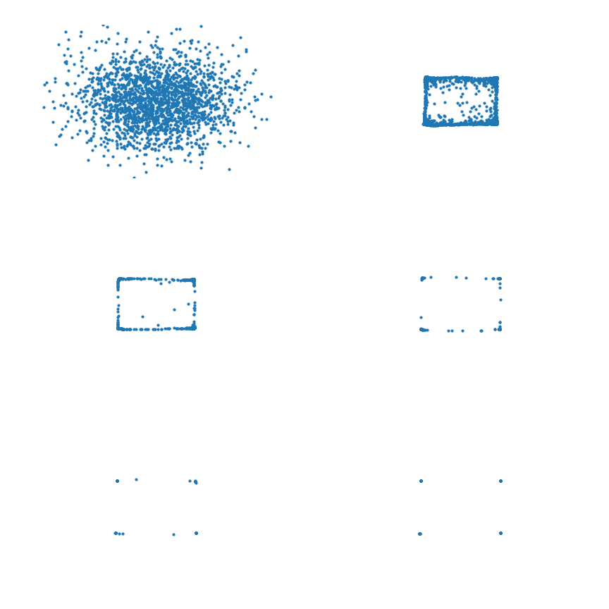
Diffusion models are supposed to be very expressive, allowing them to capture multimodalities present in the initial data. We will illustrate this with an initial data distribution being the sum of 4 narrow Gaussians with spikes at $(-1, -1)$, $(-1, 1)$, $(1, -1)$, and $(1, 1)$. As before, we will add noise until this initial distribution is indistinguishable from a Gaussian centered at the origin with std 1. The denoising process should then separate the data into the four spikes as illustrated on the gif below.

The code to implement this 2D multimodal diffusion process is simple_multimodal.py and the gif can be generated with simple_multimodal_video.py.

Denoising Diffusion Probabilistic Models (DDPM)

The diffusion models presented so far use a naive denoising process which works on our simple cases. To obtain better quality diffusion models we will follow the implementation of "Denoising Diffusion Probabilistic Models" (DDPM). The simplest code for 1D data is single_DDPM.py. Note that single_DDPM.py uses a single neural network to denoise each noise level, but we could also have one neural network for each noise level as implemented in simple_DDPM.py.

As we did previously, we can also extend DDPM to 2D multimodal data distributions with the code multimodal_DDPM.py. Finally, to get a better understanding of the evolution of the probability density functions (pdf) through the different noise scales you can look at detailed_DDPM.py.

Quick Summary

• Diffusion models learn to iteratively remove noise.
• A trained diffusion model generates new data by denoising some random initial data.
• We implemented a simple diffusion model in 100 lines of Python!

References

1. Jonathan Ho, Ajay Jain, and Pieter Abbeel, Denoising diffusion probabilistic models, Advances in Neural Information Processing Systems, pages 6840 - 6851, 2020.
2. Tero Karras, Miika Aittala, Timo Aila, and Samuli Laine, Elucidating the Design Space of Diffusion-Based Generative Models, Advances in Neural Information Processing Systems, pages 26565 - 26577, 2022.